R1.1 Incomplete Task Execution
R1.2 Deadlock due to Orientation
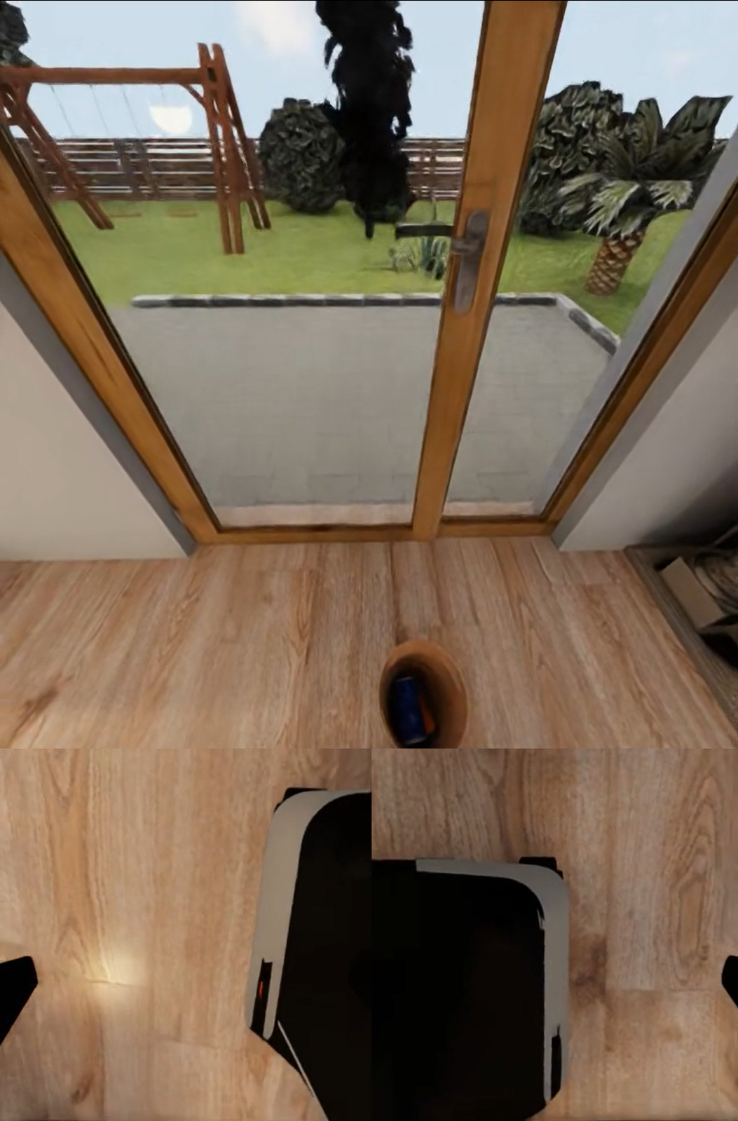
R1.3 Object Drop Failure
Supplementary Figures and Illustrations
Supplementary Video Results
When the robot moves toward the cabinet storing the hotdogs, the first potential peak appears around 25 seconds. During the attempt to open the door, the arm is oriented incorrectly, leading to the first drop in potential and a trough around 52 seconds. When the robot finds the correct way to open the door and reaches toward the hotdogs, a second potential peak appears around 74 seconds. It then picks up the first hotdog, resulting in a new potential peak around 130 seconds, and picks up the second hotdog around 160 seconds, producing a third peak. Afterward, it moves toward the microwave, with the potential remaining high. During the process of placing the hotdogs, there is a brief drop in potential, reflecting intermediate adjustments and attempts. When the robot places both hotdogs into the microwave and initiates the door-closing action, a fourth potential peak appears around 400 seconds. After further attempts, it turns on the switch around 417 seconds, reaching the final potential peak. The task is then completed, and the robot retracts its arms, causing the potential to decrease.
When the robot moves toward the cabinet storing the hotdogs, the first potential peak appears around 10 seconds. During the attempt to open the door, the arm is oriented incorrectly, leading to a trough in potential around 32 seconds. When the robot finds the correct way to open the door and reaches toward the hotdog, a second potential peak appears around 73 seconds, and the potential remains high during the door-opening process. However, when the robot attempts to grasp the hotdog, the gripper is positioned incorrectly, causing the potential to drop sharply. It then fails to pick up the hotdog, and throughout the repeated unsuccessful attempts, the potential remains at a low level.
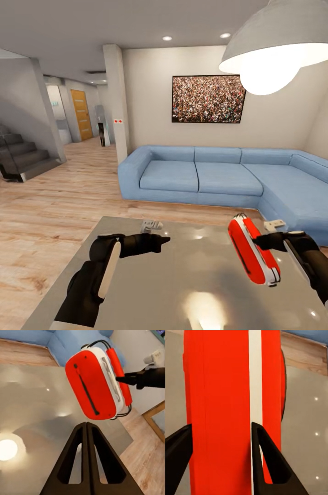
In the initial stage, the robot scans its surroundings, and the potential remains low. After locating the trash bin, it approaches and picks it up, reaching the first potential peak around 29 seconds. After a brief adjustment, it stabilizes the grasp on the trash bin, leading to a second potential peak around 41 seconds. It then moves toward the soda cans, with the potential remaining high. During the three instances of picking up the soda cans, the potential reaches smaller peaks around 67 seconds, 86 seconds, and 106 seconds. After completing the task, the robot places the trash bin on the ground, and the potential begins to decrease.
In the initial stage, the robot scans its surroundings, and the potential remains low. After locating the trash bin, it moves toward it, leading to a peak in potential. Around 43 seconds, it picks up the trash bin, reaching another peak in potential. It then approaches the soda cans, with the potential remaining high. During the two instances of picking up soda cans, the potential reaches smaller peaks around 78 seconds and 100 seconds. However, the robot forgets the existence of the third can. Around 107 seconds, it places the trash bin on the ground, resulting in a significant drop in potential, which then remains low until the episode terminates due to the time limit.
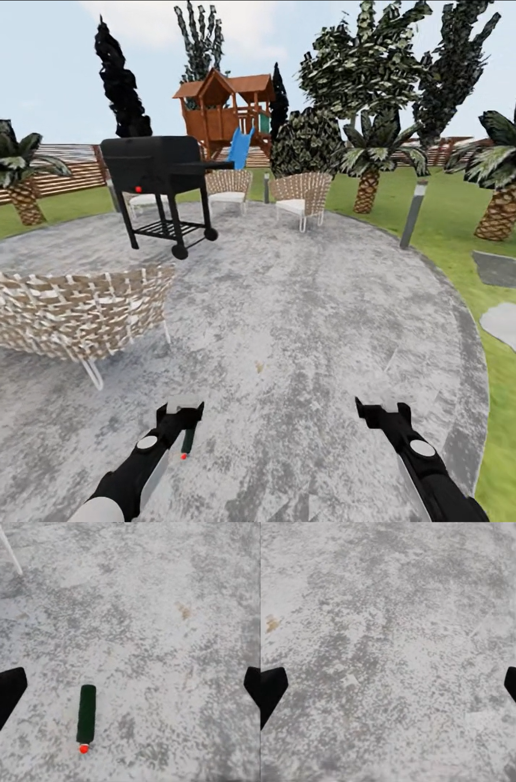
In the initial stage, the robot scans its surroundings, and the potential remains low. When it discovers and picks up the spray bottle, the potential reaches a peak around 19 seconds. It then carries the spray bottle toward the first target tree, during which the potential remains high. The potential remains at a relatively low level during the watering process. Therefore, the peak ends when the spray bottle first makes contact with the tree. After completing the first watering task, the robot turns off the spray bottle, leading to a potential peak around 105 seconds. When the robot begins moving toward the second tree, the potential rises again and remains high. Similarly, around 187 seconds, it reaches another potential peak at the moment it begins watering the tree, and the task is completed. Afterward, it continues circling around while watering, and the potential begins to decrease.
In the initial stage, the robot scans its surroundings, and the potential remains low. When it discovers and picks up the spray bottle, the potential reaches a peak around 27 seconds. However, the spray bottle slips from its grasp, causing the potential to drop sharply starting at 28 seconds. In the subsequent attempts to pick it up again, there is a brief rise in potential around 86 seconds. But the attempt fails, and the potential decreases further. After that, the robot tries to water the tree without carrying the spray bottle, so the potential remains at a low level throughout.
In the initial stage, the robot scans its surroundings, and the potential fluctuates at a low level. After locating the radio, it approaches it, leading to a peak in potential around 14 seconds. After several attempts, it picks up the radio around 27 seconds, and the potential rises rapidly. It then adjusts the position of the radio and begins trying to turn on the switch, with the potential remaining high. Around 69 seconds, it turns on the radio, reaching a peak in potential and completing the task. The subsequent process of putting the radio back is not part of the task, so the potential correspondingly decreases.
In the initial stage, the robot scans its surroundings, and the potential fluctuates at a low level. After locating the radio, it moves toward it, leading to a peak in potential around 21 seconds. However, starting at around 48 seconds, the subsequent attempts begin to deviate from a reasonable execution strategy, and the potential drops sharply. The robot then makes multiple low-quality attempts, during which the potential remains consistently low. At 142 seconds, it knocks over the radio, reaching a trough in potential. After that, it continues making low-quality attempts, and the potential stays at a low level.
In the initial stage, the robot scans its surroundings to locate and approach the washing machine, while the potential remains at a relatively high level. Around 35 seconds, it opens the washing machine door, reaching a peak in potential. After adjusting its direction, it detects the baseball caps, leading to another potential peak around 52 seconds. After several attempts, it picks up the two baseball caps around 98 seconds and 132 seconds, producing two additional potential peaks. It then places the two baseball caps into the washing machine in succession, resulting in potential peaks around 142 seconds and 161 seconds. At 188 seconds, it closes the washing machine door, reaching another potential peak. At 207 seconds, it turns on the washing machine, reaching yet another potential peak. Afterward, it retracts its arms, and the potential correspondingly decreases.
In the initial stage, the robot scans its surroundings to locate and approach the washing machine, while the potential remains at a relatively high level. Around 31 seconds, it opens the washing machine door, reaching a peak in potential. After several attempts, it picks up two baseball caps around 68 seconds and 100 seconds, producing two additional potential peaks. It then places the two baseball caps into the washing machine in succession, leading to potential peaks around 118 seconds and 132 seconds. At 226 seconds, it closes the washing machine door, reaching another potential peak. However, afterward the robot forgets to turn on the washing machine and instead continues searching for the baseball caps, causing the potential to drop rapidly and remain at a low level.
Additional Supplementary Figures
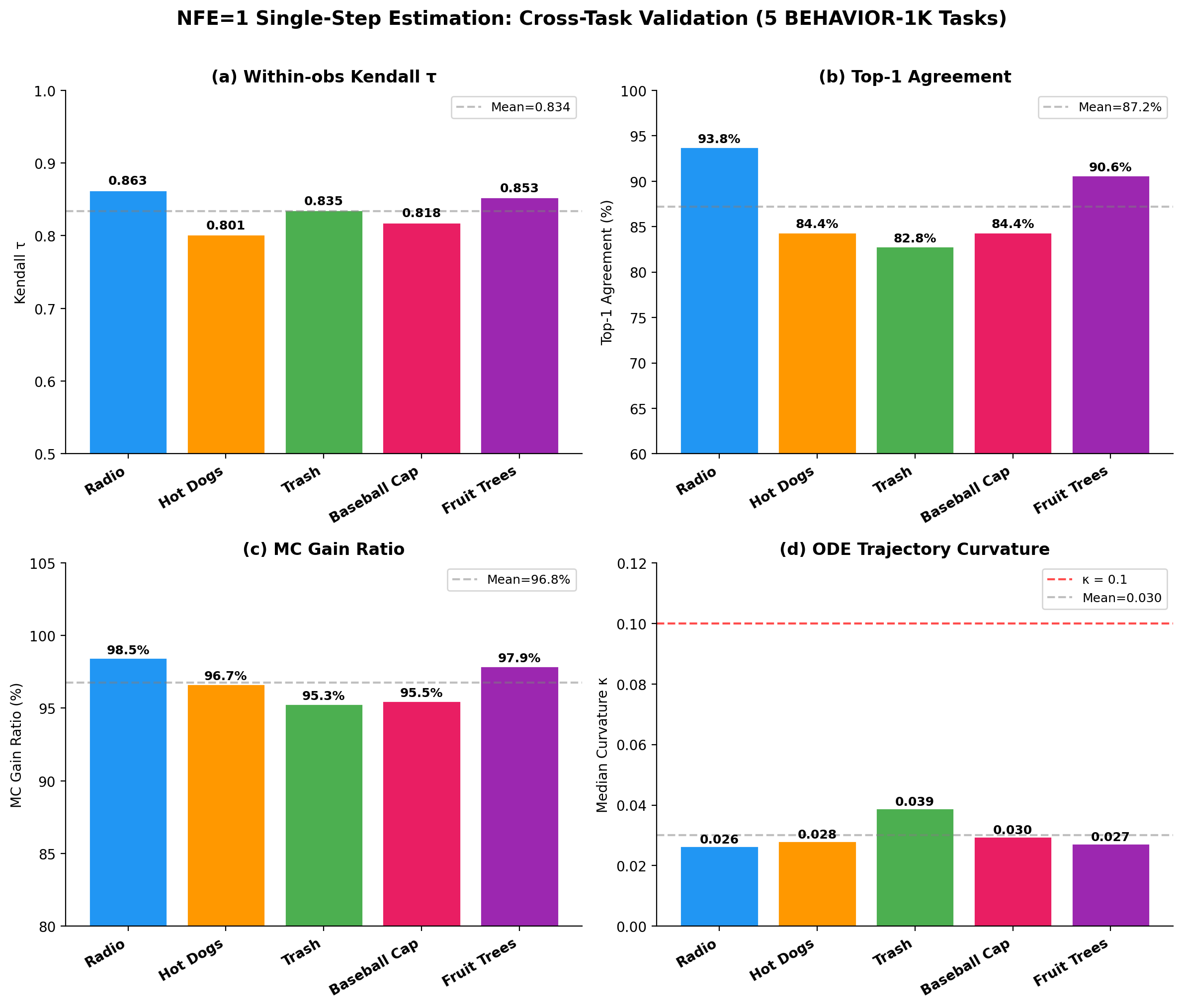
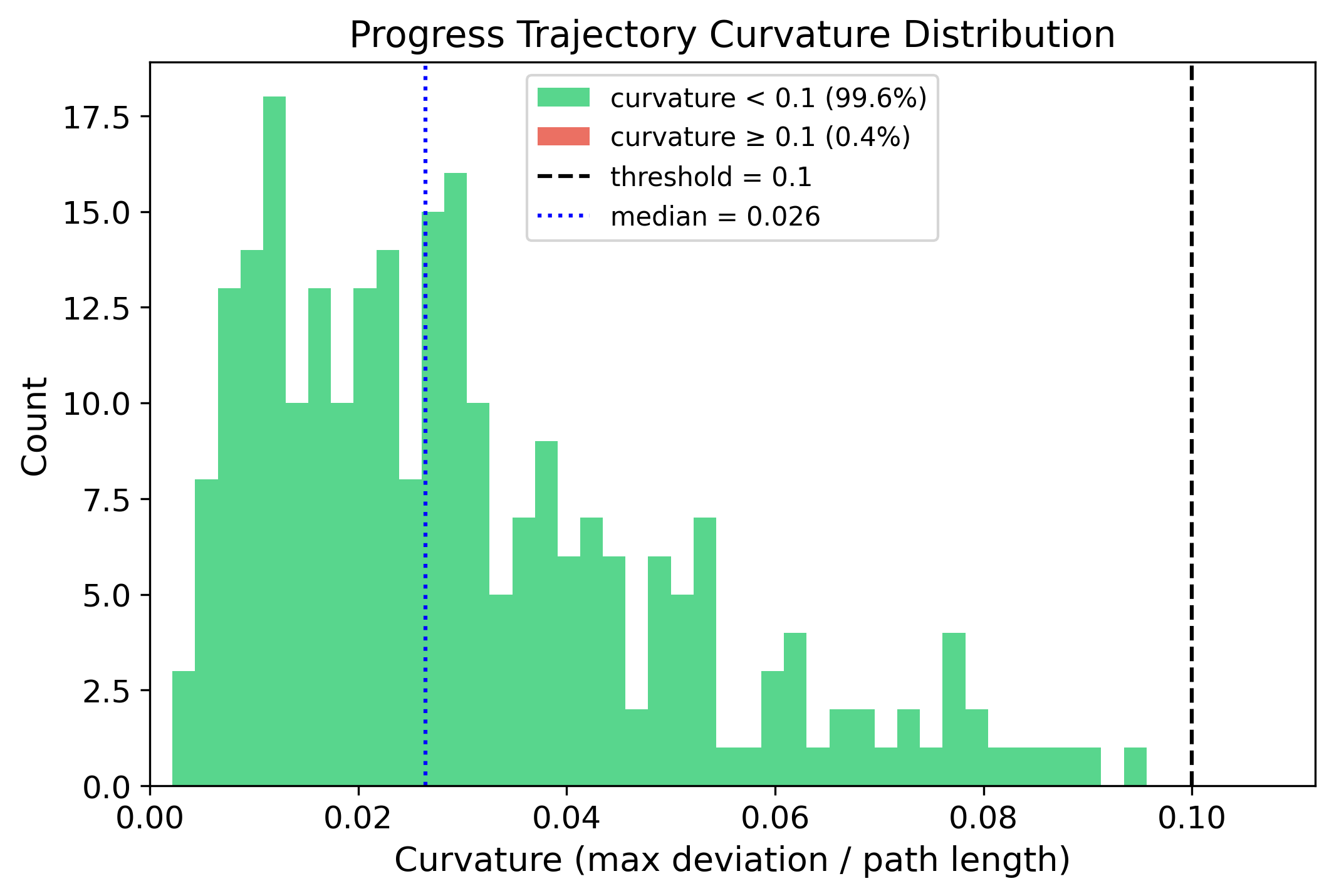
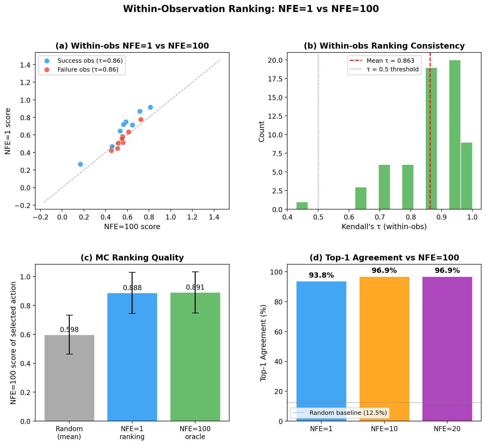
Four-panel bar chart summarizing NFE=1 single-step estimation fidelity across five BEHAVIOR-1K tasks (Turning on radio, Cook hot dogs, Picking up trash, Wash a baseball cap, Spraying fruit trees). **(a) Within-observation Kendall τ** (NFE=1 vs. NFE=100): range [0.801, 0.863], mean 0.834 (dashed line). **(b) Top-1 Agreement** (fraction of observations where NFE=1 and NFE=100 select the same best candidate): range [82.8%, 93.8%], mean 87.2%. **(c) MC Gain Ratio** (MC sampling benefit under NFE=1 relative to NFE=100): range [95.3%, 98.5%], mean 96.8%. **(d) ODE Trajectory Curvature κ** (median per task): range [0.026, 0.039], mean 0.030; all values fall well below the κ=0.1 threshold (red dashed line).
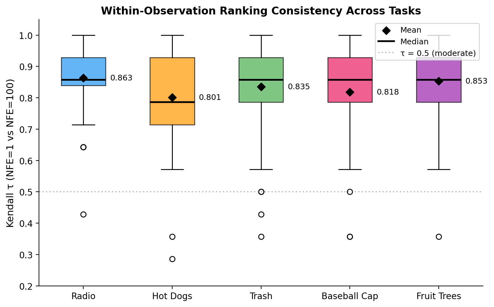
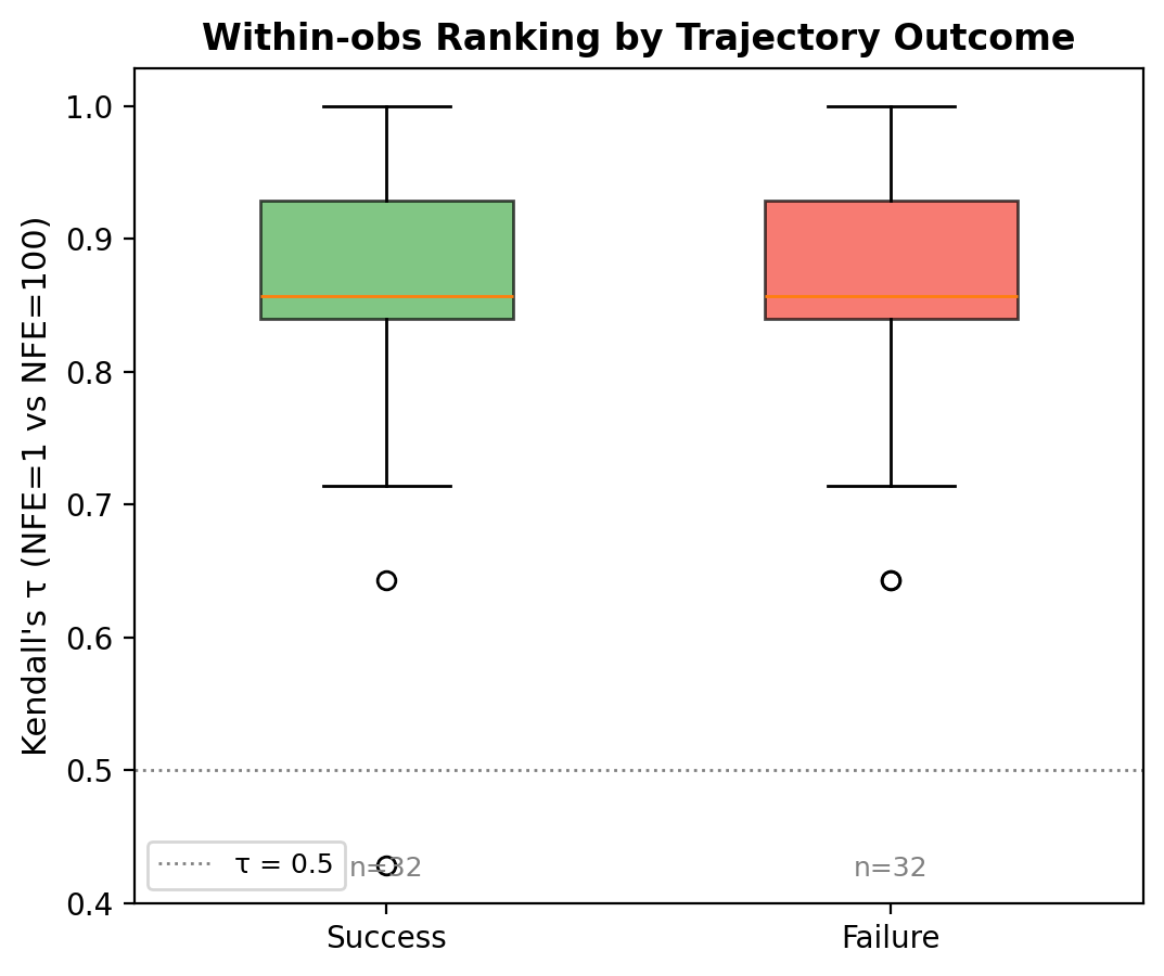
Box plot of per-observation Kendall τ distributions across 64 stratified-sampled observations (32 success + 32 failure, K=8 candidates each) for each of five tasks. Boxes span Q1–Q3; diamonds mark the mean; black horizontal lines indicate the median; open circles denote outliers. The gray dashed line at τ=0.5 marks the random-ordering baseline. All five tasks achieve mean τ > 0.80, with interquartile ranges concentrated in the high-fidelity region (τ > 0.7), indicating that NFE=1 preserves relative action ranking quality consistently across tasks.
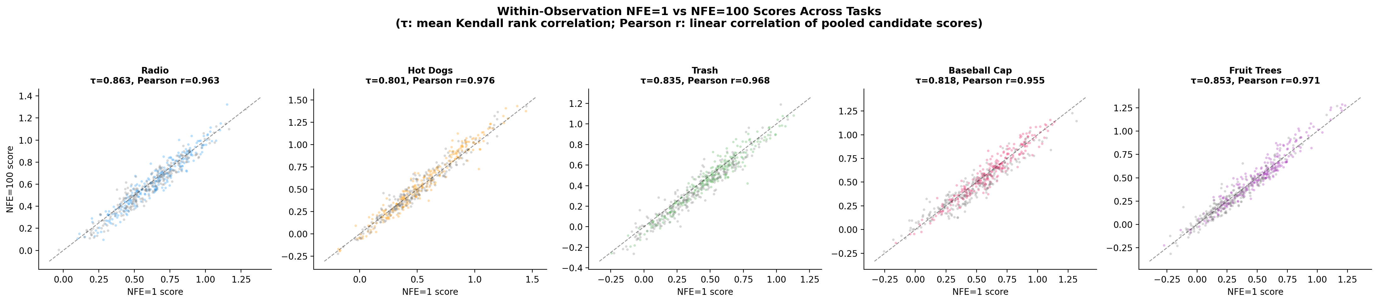
Scatter plots comparing NFE=1 predicted progress scores (x-axis) against NFE=100 reference scores (y-axis) for all (observation, candidate) pairs, shown separately for each of five tasks (64 stratified-sampled observations per task, 32 success + 32 failure, K=8 candidates each; 512 points per subplot). Each subplot title reports the task-level Kendall τ and Pearson r (computed over K=8 candidates pooled across all 64 observations): Turning on radio τ=0.863, r=0.963; Cook hot dogs τ=0.801, r=0.976; Picking up trash τ=0.835, r=0.968; Wash a baseball cap τ=0.818, r=0.955; Spraying fruit trees τ=0.853, r=0.971. All tasks show diagonal alignment, showing linear correspondence between NFE=1 and NFE=100 estimates.

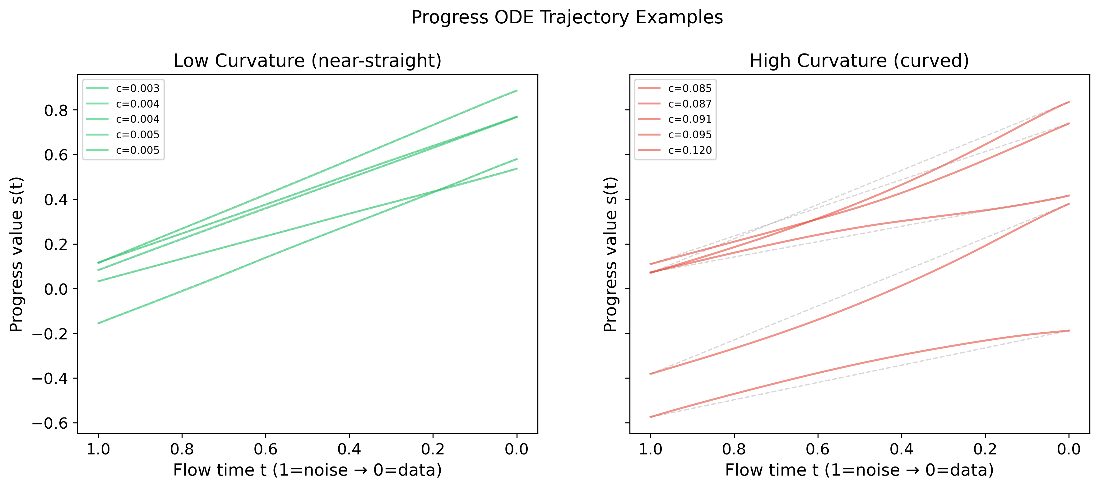
10×5 panel of ODE solution trajectories (one column per task; flow time t from 1=noise to 0=data; y-axis shows the progress score dimension s(t); colors distinguish observations). The top five rows show the five lowest-curvature trajectories per task; the bottom five rows show the five highest-curvature trajectories.
We thank all reviewers for the constructive feedback across both rounds of discussion. Below we present the planned revisions for the camera-ready manuscript. Section Summary of Key Revisions summarizes the most important changes addressing the key concerns raised by Reviewers 2 and 4. Section Complete Revision Plan provides the complete revision plan with exact original and replacement text for every modification.
The revision involves edits across Abstract, Introduction, Preliminaries, Method, Experiments, Conclusion, and Appendix. The changes fall into four categories.
Concern. The paper cited OT-CFM (optimal-transport conditional flow matching) to justify the one-step estimator, but the implementation uses standard CFM with independent noise-data sampling, not OT coupling. Theorem A.1's original premise was therefore incorrect.
Revision.
Theorem [Success Potential Recovery under Conditional FM]
Consider conditional flow matching with independent noise-data sampling, where \(\mathbf{x}_0 \sim p_0\) and \(\mathbf{x}_1 \sim p_{\text{data}}(\cdot | \mathbf{c})\) are drawn independently for each context \(\mathbf{c}\), and deterministic linear interpolation \(\mathbf{x}_\sigma = (1-\sigma)\mathbf{x}_0 + \sigma \mathbf{x}_1\) (zero path variance). Define the population-level optimal velocity field as the conditional expectation:
$$ \mathbf{v}^*(\mathbf{x}, \sigma, \mathbf{c}) \triangleq \mathbb{E}[\mathbf{x}_1 - \mathbf{x}_0 \mid \mathbf{x}_\sigma = \mathbf{x}, \mathbf{c}], $$which coincides with the \(L^2\) minimiser of \(\mathcal{L}_{\mathrm{CFM}}\) for \(\sigma\)-a.e. in the training distribution. Then at \(\sigma = 0\):
$$ \mathbf{x}_0 + \mathbf{v}^*(\mathbf{x}_0, 0, \mathbf{c}) = \mathbb{E}_{\mathbf{x}_1 \sim p_{\text{data}}(\cdot|\mathbf{c})}[\mathbf{x}_1] \quad \text{for } p_0\text{-a.e. } \mathbf{x}_0. $$In particular, the progress component recovers the dataset-conditional success probability \(\mathbb{E}[y \mid \mathbf{c}] = P_{\mathcal{D}}(\mathrm{Success} \mid \mathbf{c})\).
The CFM objective minimizes the regression loss:
$$ \mathcal{L}_{\text{CFM}}(\theta) = \mathbb{E}_{\sigma, \mathbf{x}_0, \mathbf{x}_1} \left[ \| \mathbf{v}_\theta(\mathbf{x}_\sigma, \sigma, \mathbf{c}) - (\mathbf{x}_1 - \mathbf{x}_0) \|^2 \right]. $$By definition, \(\mathbf{v}^*\) is the population-level \(L^2\) minimizer, i.e., the conditional expectation:
$$ \mathbf{v}^*(\mathbf{x}, \sigma, \mathbf{c}) = \mathbb{E}_{\mathbf{x}_0, \mathbf{x}_1} \left[ \mathbf{x}_1 - \mathbf{x}_0 \mid \mathbf{x}_\sigma = \mathbf{x}, \mathbf{c} \right]. $$At \(\sigma=0\), the deterministic linear interpolation gives \(\mathbf{x}_{\sigma=0} = \mathbf{x}_0\). Substituting:
$$ \mathbf{v}^*(\mathbf{x}_0, 0, \mathbf{c}) = \mathbb{E}_{\mathbf{x}_1} \left[ \mathbf{x}_1 - \mathbf{x}_0 \mid \mathbf{x}_0, \mathbf{c} \right] = \mathbb{E}[\mathbf{x}_1 \mid \mathbf{x}_0, \mathbf{c}] - \mathbb{E}[\mathbf{x}_0 \mid \mathbf{x}_0, \mathbf{c}]. $$Since \(\mathbf{x}_0 \perp \mathbf{x}_1 \mid \mathbf{c}\) (independent noise-data sampling), the conditional expectation simplifies to the marginal:
$$ \mathbb{E}[\mathbf{x}_1 \mid \mathbf{x}_0, \mathbf{c}] = \mathbb{E}_{\mathbf{x}_1 \sim p_{\text{data}}(\cdot|\mathbf{c})} [\mathbf{x}_1 \mid \mathbf{c}]. $$Since \(\mathbb{E}[\mathbf{x}_0 \mid \mathbf{x}_0, \mathbf{c}] = \mathbf{x}_0\):
$$ \mathbf{v}^*(\mathbf{x}_0, 0, \mathbf{c}) = \mathbb{E}[\mathbf{x}_1 \mid \mathbf{c}] - \mathbf{x}_0. $$Therefore:
$$ \hat{\mathbf{x}}_1 = \mathbf{x}_0 + \mathbf{v}^*(\mathbf{x}_0, 0, \mathbf{c}) = \mathbb{E}[\mathbf{x}_1 \mid \mathbf{c}]. $$For the success potential component, the target is the broadcasted binary outcome \(y \in \{0, 1\}\):
$$ \mathbb{E}[y \mid \mathbf{c}] = P_{\mathcal{D}}(\text{Success} \mid \mathbf{c}). $$The theorem characterizes \(\mathbf{v}^*\) (the population conditional expectation), not the learned \(\mathbf{v}_\theta\). In practice, finite network capacity means \(\mathbf{v}_\theta\) only approximates \(\mathbf{v}^*\). We assess this gap empirically: cross-state correlation with NFE=20 yields \(\rho = 0.997\) (Turning on Radio); within-observation Kendall \(\tau\) (NFE=1 vs. NFE=100) yields \(0.863\) on Turning on Radio and ranges from \(0.801\) to \(0.863\) across five tasks (mean \(0.834\)), confirming that single-step estimates preserve relative sample ordering.
Concern. Decoupled AWR was presented as a key conceptual contribution, but decoupling policy and value losses is standard in separated actor-critic architectures. The one-step estimator's positioning as a “value estimator” was overclaimed.
Revision.
Concern. The paper was hard to understand for readers outside the robotics subcommunity. The motivation for decoupled weighting was not intuitive.
Revision.
Revision.
Below we list every planned modification with exact location, original text, and replacement text. Changes are grouped by paper section. Red strikethrough marks removed text; green marks new text.
Original:
Furthermore, by exploiting the straight-path structure of optimal-transport conditional flow matching, we derive a single-step value estimator that computes advantages in a single forward pass, making RL fine-tuning computationally comparable to supervised learning. We prove theoretically the consistency of this estimator ...
Revised:
Furthermore, we propose a low-cost one-step baseline proxy that computes advantages in a single forward pass, motivated by the population-level conditional-mean property of the flow matching regression objective under independent noise-data sampling. This makes RL fine-tuning computationally comparable to supervised learning. ...
L156. consistent → corresponding quality estimate.
L158. unbiased calibration → calibrated value estimation.
L167. we exploit a structural property of optimal-transport conditional flow matching: the optimal transport path is a straight line ... → we use a one-step proxy at the noise boundary as a low-cost baseline estimator, motivated by the population-level conditional-mean property of the flow matching regression objective under independent noise-data sampling.
Contribution #2 title (L184). efficient value estimation → efficient baseline estimation.
Contribution #2 text (L185). We introduce ... we further derive a single-step value estimator → We employ a decoupled AWR objective ... and adopt a low-cost one-step baseline proxy, which is empirically validated for test-time self-guidance.
Contribution #3 (L187). a effective → an effective.
L215. \(v_\theta\) → \(\mathbf{v}_\theta\) (notation fix). L219: \(\mathcal{u}_\sigma\) → \(\mathbf{u}_\sigma\).
L215. optimal transport probability path → standard linear interpolation path.
L225. single-step value estimation → baseline estimation.
Section 3 opening (L248, new). Added method overview paragraph:
FPF is built around three design choices. First, we augment the flow-matching backbone with a per-step progress head: rather than maintaining a separate critic network, the shared backbone jointly generates action sequences and predicts a scalar success potential at each step, using all intermediate representations. Second, we train the two heads with decoupled supervision: the action head is weighted by AWR importance weights \(w = \min(M, \exp(A/\tau))\) to reinforce high-advantage transitions, while the progress head is always trained with unit weight, preventing gradient masking on low-advantage (typically failure) data where \(w \approx 0\) would otherwise starve the progress head of corrective signal. Third, we estimate the per-sample advantage baseline via a one-step proxy: a single forward pass at the noise boundary \(\sigma = 0\), rather than full ODE integration, provides the baseline \(\hat{V}\), reducing training cost to that of standard supervised learning. The following subsections describe each choice in detail.
L255. intrinsic estimator of \(P(\text{success} | \mathbf{c}, \mathbf{a})\) → learned scoring signal. At the population level, it recovers \(P_\mathcal{D}(\text{success} | \mathbf{c})\).
L260 (new). Added per-step design rationale:
We note that per-step modeling is a design choice rather than a uniquely justified option. Since the backbone already produces step-wise action features, attaching the progress head at each step is the most natural integration point and avoids introducing an additional temporal aggregation module. A per-chunk scalar head is also feasible, and may be sufficient in settings where only chunk-level supervision is available.
L263. we introduce → we employ.
L279. Section title: Single-Step State-Value Estimation → Single-Step Baseline Proxy.
L282--291.
Instead, we propose single-step state-value estimation that leverages the property of optimal-transport conditional flow matching (OT-CFM)~[flow_matching]: the OT probability path is a straight line between noise and data a single-step baseline estimation that exploits the conditional-mean property of the flow matching regression objective. Under deterministic linear interpolation
$$ \mathbf{x}_\sigma = (1-\sigma)\mathbf{x}_0 + \sigma \mathbf{x}_1, \quad \sigma \in [0,1], $$with target velocity \(\mathbf{u}_\sigma = \mathbf{x}_1 - \mathbf{x}_0\), CFM training minimizes a squared-loss regression objective. At the population optimum of this objective, the predicted velocity matches whose population-level \(L^2\) minimizer is the conditional mean of the target velocity given \((\mathbf{x}_\sigma,\sigma,\mathbf{c})\).
In particular, at \(\sigma=0\) we have \(\mathbf{x}_{\sigma}=\mathbf{x}_0\) and \(\mathbf{x}_0\) is independent of \(\mathbf{x}_1\), which motivates the simplification: At \(\sigma=0\), the flow state reduces to pure noise \(\mathbf{x}_{\sigma}=\mathbf{x}_0\). Since noise and data are sampled independently (\(\mathbf{x}_0 \perp \mathbf{x}_1 \mid \mathbf{c}\)), the optimal velocity simplifies to:
$$ \mathbf{v}^*(\mathbf{x}_0,0,\mathbf{c})=\mathbb{E}[\mathbf{x}_1| \mathbf{c}]-\mathbf{x}_0. $$L301. theoretically grounded ... recovers true expected value → motivated by the population-level conditional-mean property of the CFM regression objective under independent sampling, and empirically validated: cross-state \(\rho = 0.997\) (NFE=20, Turning on Radio); within-observation Kendall \(\tau\) ranges from \(0.801\) to \(0.863\) across five tasks (mean \(0.834\), NFE=100).
Figure 2 caption (L307). Two changes: Single-step value estimation → Single-step baseline proxy; unbiased calibration → calibrated value estimation.
L329 (new text after). Added numerical walkthrough: “For example, with \(A = -2.0\) and \(\tau = 0.5\), the AWR weight is \(w = \exp(-4) \approx 0.018\) ...”
L329. unbiased value learning → calibrated value learning.
L339. Added: “The effectiveness of this test-time ranking is validated empirically in Section 4.3.”
L394. Approximation validity → Approximation quality; single-step estimator → single-step proxy.
L473. validity of the efficient single-step value estimator → practical fidelity of the single-step baseline proxy.
Figure 6 (L523, L526). single-step state-value estimation / single-step approximation → single-step baseline proxy / practical fidelity of the single-step proxy.
L530--531. Efficiency of single-step state-value estimation / single-step estimator → Efficiency of single-step baseline estimation / single-step proxy.
Restructured to: (1) unified architecture as primary contribution; (2) decoupled supervision and one-step baseline as practical design choices; (3) expanded limitations covering stage-level binary rewards and explicit scope (\(5 + 5\) tasks, Pi0/Pi0.5, \(\tau \in \{0.3, 0.5, 0.7\}\), \(K \in \{1, 5, 10\}\), NFE \(\in \{1, 20\}\)).
New Broader Impact paragraph (added after Conclusion):
Progress in generalizable robot learning may improve efficiency and safety in physical tasks, but also risks labor displacement in sectors such as manufacturing, logistics, and domestic work. The best-of-\(K\) test-time ranking mechanism could amplify biases present in the training data, as it preferentially selects action patterns that score highly under the learned progress head; if the training distribution is skewed, the ranking may systematically favor certain behaviors. Responsible deployment should include ongoing safety monitoring, evaluation of failure modes in out-of-distribution environments, and consideration of the social and economic contexts in which the system is used.
L575. theoretically grounded → population-level properties.
L580. Section title: Consistency of Success Potential Learning → Population-Level Properties of Success Potential.
L583. proxy for the value function → proxy for the dataset-conditional success probability.
L585--612. Theorem A.1 fully restated (see Section above). Proof Step 3 now explicitly states \(\mathbf{x}_0 \perp \mathbf{x}_1 \mid \mathbf{c}\).
L609. strictly defined as the state value function → Under standard assumptions, this coincides with \(V^{\pi_\beta}(\mathbf{c})\).
L611. unbiased estimator of \(V^{\pi_\beta}\) → recovers \(P_\mathcal{D}(\text{Success} \mid \mathbf{c})\) at the population level.
L614--617. Remark A.2 fully rewritten (see Section above).
L656. A key contribution → A practical design choice.
L691. unbiased critic → calibrated scoring proxy.
L744. performing a Monte Carlo approximation of \(\pi^*\) → performing approximate best-of-\(K\) selection, ranking by predicted quality score \(Q^{(k)}\).